Getting Started

This notebook walks through the main combatlearn features: classic ComBat (Johnson et al. 2007), neuroComBat (Fortin et al. 2018), CovBat (Chen et al. 2022), Longitudinal ComBat (Beer et al. 2020), and ComBat-GAM (Pomponio et al. 2020).

pip install combatlearn

import warnings

warnings.filterwarnings("ignore")

import numpy as np
import pandas as pd
import matplotlib.pyplot as plt
from sklearn.decomposition import PCA
from sklearn.model_selection import cross_val_score, train_test_split, GridSearchCV
from sklearn.pipeline import Pipeline
from sklearn.preprocessing import StandardScaler
from sklearn.linear_model import LogisticRegression
from sklearn.svm import SVC

from combatlearn import ComBat
from combatlearn.visualization import plot_transformation, plot_feature_diagnostics, plot_batch_effect_heatmap
from combatlearn.metrics import compute_batch_metrics
from combatlearn.inspection import feature_batch_diagnostics, summary

plt.rcParams["figure.dpi"] = 120

def plot_pca(X, labels, title):
    pca = PCA(n_components=2)
    pts = pca.fit_transform(X)
    _ = plt.figure(dpi=150)
    for b in np.unique(labels):
        idx = labels == b
        plt.scatter(pts[idx, 0], pts[idx, 1], label=f"batch {b}")
    plt.title(title)
    plt.xlabel("PC1")
    plt.ylabel("PC2")
    plt.legend()
    plt.show()

Simulating data

rng = np.random.default_rng(42)

n_samples, n_features, n_batches = 300, 50, 3
true_signal = rng.standard_normal((n_samples, n_features))

# Feature-specific batch effects: first 15 features have strong effects,
# next 15 moderate, remaining 20 have weak/no effects
feature_strength = np.concatenate([
    np.ones(15) * 3.0,
    np.ones(15) * 1.0,
    np.ones(20) * 0.1,
])

batch_effects = rng.normal(
    loc=np.array([0, 3, -2])[:, None] * feature_strength[None, :],
    scale=0.3,
    size=(n_batches, n_features),
)

batches = np.repeat(np.arange(n_batches), n_samples // n_batches)
X = true_signal.copy()

for b in range(n_batches):
    X[batches == b] += batch_effects[b]

X = pd.DataFrame(X, columns=[f"gene_{i + 1}" for i in range(n_features)])
batch_labels = pd.Series(batches.astype(str), name="batch")

sex = pd.Series(rng.choice(["M", "F"], size=n_samples), name="sex")
age = pd.Series(rng.uniform(20, 60, size=n_samples), name="age")

y = (true_signal[:, 0] > 0).astype(int)

plot_pca(X.values, batch_labels.values, title="Before correction")

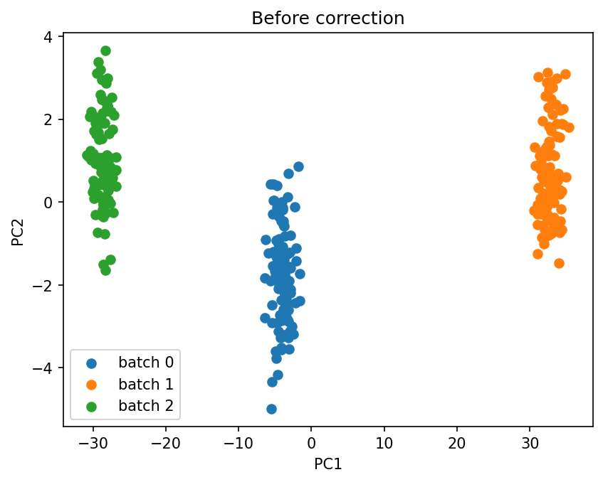
The methods

combatlearn exposes every variant through the same ComBat estimator; you pick one with the method argument. The sections below build up from the original algorithm to its covariate-aware, high-dimensional, longitudinal, and nonlinear extensions.

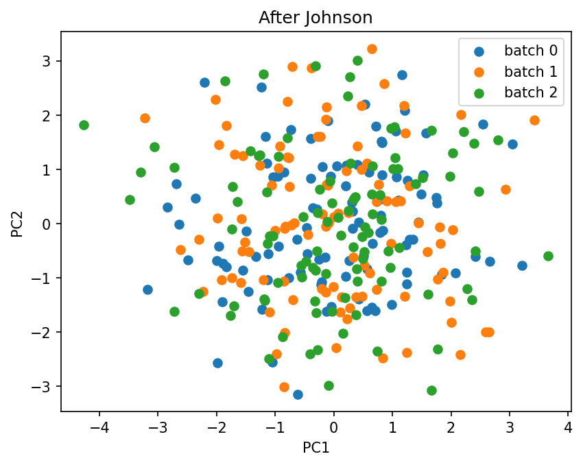
Johnson method

The johnson method (Johnson et al., 2007) is the original ComBat. It standardizes each feature, estimates per-batch location (mean) and scale (variance) shifts, and pools them across features with empirical Bayes shrinkage before removing them. It corrects batch effects only and ignores covariates, which makes it the simplest and fastest option when there is no biological signal to preserve.

We apply it to the simulated data and compare the PCA before and after correction.

combat_johnson = ComBat(batch=batch_labels, method="johnson")
X_johnson = combat_johnson.fit_transform(X)

plot_pca(X_johnson.values, batch_labels.values, title="After Johnson")

Because the johnson method has no covariate support, passing discrete_covariates or continuous_covariates leaves the result unchanged, as the check below confirms.

combat_johnson_wc = ComBat(
    batch=batch_labels,
    discrete_covariates=sex,
    continuous_covariates=age,
    method="johnson",
)
X_johnson_wc = combat_johnson_wc.fit_transform(X)
print("Are all values equal?", "Yes" if np.allclose(X_johnson, X_johnson_wc) else "No")

Are all values equal? Yes

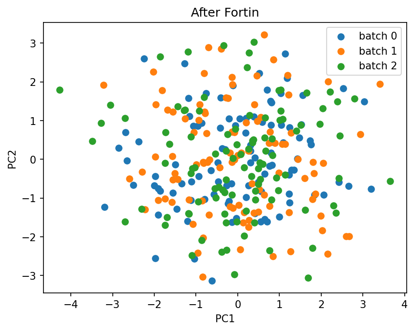
Fortin method

The fortin method (Fortin et al., 2018), also known as neuroComBat, extends Johnson by bringing the covariates into the model. It fits a design matrix of batch indicators plus covariates, so the covariate effects (here sex and age) are preserved while only the batch-related variation is removed. This is the recommended default whenever biological variables are known.

We correct the same data, this time passing the covariates.

combat_fortin = ComBat(
    batch=batch_labels,
    discrete_covariates=sex,
    continuous_covariates=age,
    method="fortin",
)
X_fortin = combat_fortin.fit_transform(X)

plot_pca(X_fortin.values, batch_labels.values, title="After Fortin")

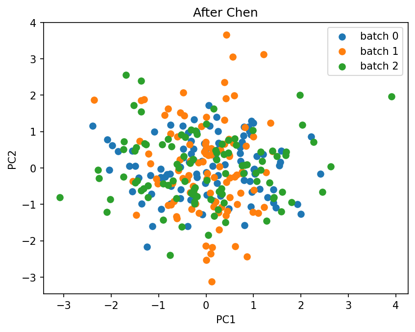
Chen method

The chen method (Chen et al., 2022), also known as CovBat, extends Fortin by harmonizing the covariance structure on top of the mean and variance. After the Fortin step it runs PCA on the residuals and applies a second batch correction in principal-component space, removing batch effects that show up as differences in feature-to-feature correlations. covbat_cov_thresh sets how much variance the PCA step keeps: a float for cumulative variance (e.g. 0.95), or an int for a fixed number of components.

We correct the data with covariates and 95% of the variance retained.

combat_chen = ComBat(
    batch=batch_labels,
    discrete_covariates=sex,
    continuous_covariates=age,
    method="chen",
    covbat_cov_thresh=0.95,
)
X_chen = combat_chen.fit_transform(X)

plot_pca(X_chen.values, batch_labels.values, title="After Chen")

Longitudinal method

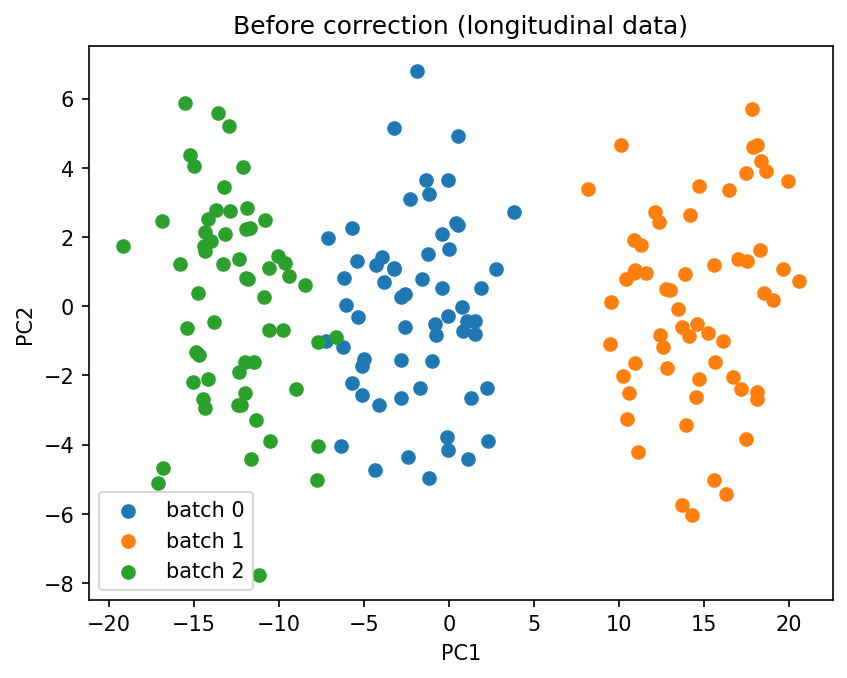
The longitudinal method (Beer et al., 2020) targets repeated-measures designs, where the same subjects are measured more than once (e.g. across visits or sites). It extends the Fortin model with a per-subject random intercept - a subject-specific offset shared across that subject’s repeated measurements - so within-subject correlation is modelled rather than treated as noise. It requires a subject_id (one label per sample) and accepts an optional time_covariate.

The data simulated above is cross-sectional, so here we build a small longitudinal dataset: each subject is measured at several visits, with the visits spread across batches.

# Build a small longitudinal dataset: subjects measured at multiple visits across batches
n_subjects, n_visits, n_long_features = 60, 3, 30
batch_levels = ["0", "1", "2"]
batch_shifts = {"0": 0.0, "1": 3.0, "2": -2.0}

subject_intercepts = rng.standard_normal((n_subjects, n_long_features)) * 1.5

records, subjects_long, visits_long, batches_long = [], [], [], []
for s in range(n_subjects):
    for t in range(n_visits):
        b = batch_levels[(s + t) % len(batch_levels)]
        records.append(rng.standard_normal(n_long_features) + subject_intercepts[s] + batch_shifts[b] + 0.5 * t)
        subjects_long.append(f"subj_{s}")
        visits_long.append(float(t))
        batches_long.append(b)

X_long = pd.DataFrame(np.array(records), columns=[f"gene_{i + 1}" for i in range(n_long_features)])
batch_long = pd.Series(batches_long, name="batch")
subject_long = pd.Series(subjects_long, name="subject")
visit_long = pd.Series(visits_long, name="visit")

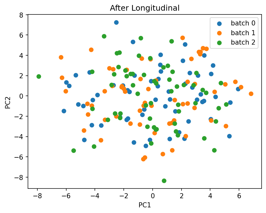
combat_long = ComBat(
    batch=batch_long,
    subject_id=subject_long,
    time_covariate=visit_long,
    method="longitudinal",
)
X_long_corrected = combat_long.fit_transform(X_long)

plot_pca(X_long.values, batch_long.values, title="Before correction (longitudinal data)")
plot_pca(X_long_corrected.values, batch_long.values, title="After Longitudinal")

GAM methods (ComBat-GAM)

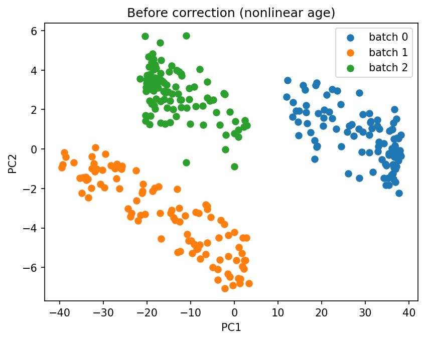
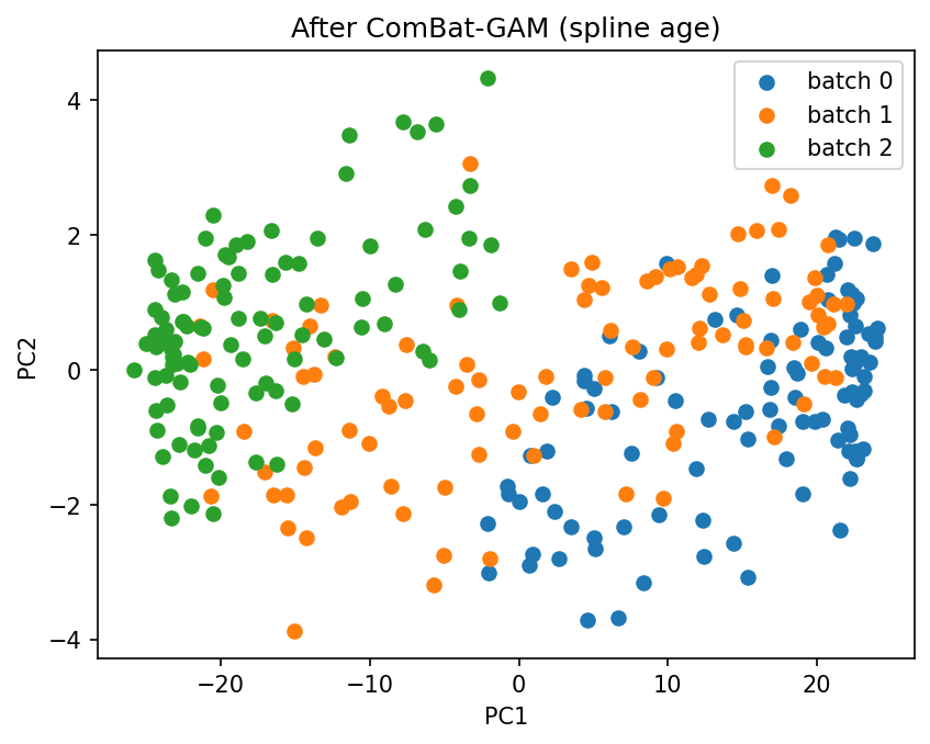
The gam method (Pomponio et al., 2020) extends Fortin by modelling continuous covariates nonlinearly with B-splines, instead of assuming a linear effect. This matters when a covariate such as age has a curved relationship with the features - especially when it is also correlated with batch, where a linear model would confound the nonlinear covariate effect with the batch effect. method="covbat_gam" applies the same spline model inside CovBat. Like Fortin/Chen, the GAM methods are inductive and cross-validation-safe.

Below we build data with a nonlinear age effect whose range differs by batch, then compare Fortin (linear age) with ComBat-GAM (spline age).

# Data with a nonlinear age effect, with age range correlated with batch
n_gam, n_gam_features = 300, 30
age_gam = rng.uniform(20, 80, n_gam)
tertiles = np.quantile(age_gam, [1 / 3, 2 / 3])
batch_gam = np.where(age_gam < tertiles[0], "0", np.where(age_gam < tertiles[1], "1", "2"))
age_curve = np.sin((age_gam - 20) / 60 * 2 * np.pi)  # nonlinear lifespan effect
loadings = rng.uniform(0.5, 1.5, n_gam_features)
gam_shifts = {"0": 3.0, "1": -3.0, "2": 1.0}
batch_shift_gam = np.array([gam_shifts[b] for b in batch_gam])[:, None]

# The batch-free signal we want to recover (nonlinear age effect + noise), before the batch shift
oracle_gam = 4.0 * np.outer(age_curve, loadings) + rng.standard_normal((n_gam, n_gam_features))
X_gam = pd.DataFrame(
    oracle_gam + batch_shift_gam,
    columns=[f"gene_{i + 1}" for i in range(n_gam_features)],
)
batch_gam = pd.Series(batch_gam, name="batch")
age_gam_df = pd.DataFrame({"age": age_gam})

X_gam_fortin = ComBat(
    batch=batch_gam, continuous_covariates=age_gam_df, method="fortin"
).fit_transform(X_gam)
X_gam_corrected = ComBat(
    batch=batch_gam, continuous_covariates=age_gam_df, method="gam"
).fit_transform(X_gam)

plot_pca(X_gam.values, batch_gam.values, title="Before correction (nonlinear age)")
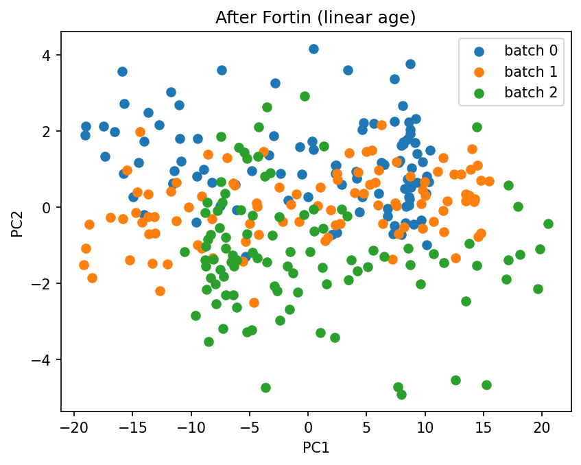
plot_pca(X_gam_fortin.values, batch_gam.values, title="After Fortin (linear age)")
plot_pca(X_gam_corrected.values, batch_gam.values, title="After ComBat-GAM (spline age)")

def recovery_mse(corrected, oracle):
    """MSE to the batch-free signal after removing the global offset (lower = better)."""
    c = corrected.values - corrected.values.mean(axis=0)
    o = oracle - oracle.mean(axis=0)
    return float(((c - o) ** 2).mean())


print("Recovery MSE vs the batch-free signal (lower is better):")
print(f"  Fortin (linear age):     {recovery_mse(X_gam_fortin, oracle_gam):.3f}")
print(f"  ComBat-GAM (spline age): {recovery_mse(X_gam_corrected, oracle_gam):.3f}")

Recovery MSE vs the batch-free signal (lower is better):
  Fortin (linear age):     5.800
  ComBat-GAM (spline age): 0.118

Fortin mixes the batches only by deleting real age signal along with the batch shift (age is confounded with batch here), so it looks cleaner in PCA but scores far worse against the batch-free signal. Batch overlap in a PCA is a trustworthy check only when batch is not confounded with a covariate you want to keep.

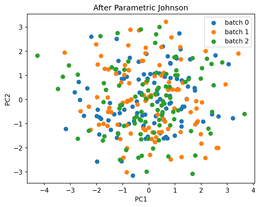
Parametric versus non-parametric approach

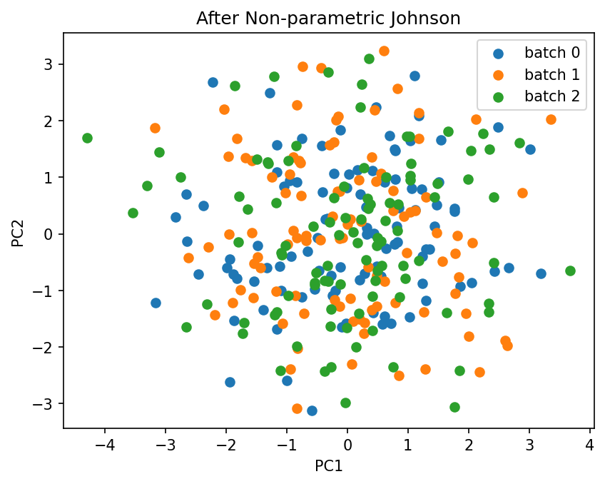
Every method estimates its per-batch parameters with empirical Bayes, in one of two modes. Parametric (the default, parametric=True) assumes the batch effects follow normal and inverse-gamma priors, which is fast and works well for most datasets. Non-parametric (parametric=False) drops the distributional assumption and estimates the priors directly from the data with an iterative scheme; it is more robust when the parametric assumptions are violated, at some extra computational cost.

Below we run both on the same data and compare the PCA.

combat_parametric = ComBat(batch=batch_labels, method="johnson", parametric=True)
X_parametric = combat_parametric.fit_transform(X)
plot_pca(X_parametric.values, batch_labels.values, title="After Parametric Johnson")

combat_non_parametric = ComBat(batch=batch_labels, method="johnson", parametric=False)
X_non_parametric = combat_non_parametric.fit_transform(X)
plot_pca(X_non_parametric.values, batch_labels.values, title="After Non-parametric Johnson")

Working with scikit-learn

Train / test split

X_train, X_test, y_train, y_test = train_test_split(
    X, y, test_size=0.2, random_state=42
)

combat = ComBat(batch=batch_labels, method="johnson")
combat.fit(X_train)

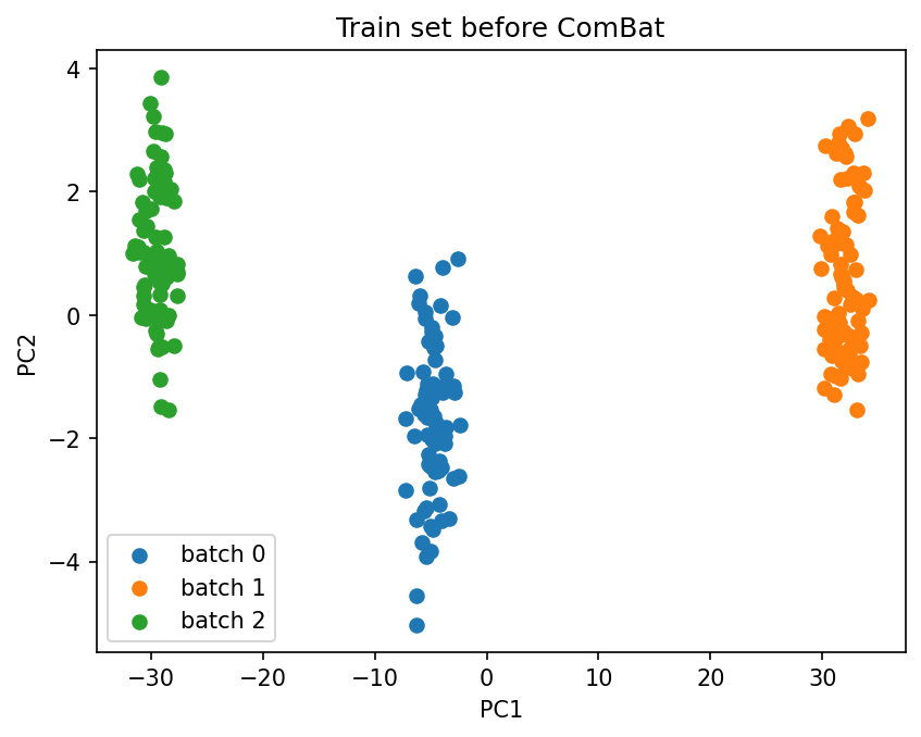
plot_pca(
    X_train.values,
    batch_labels.iloc[X_train.index].values,
    title="Train set before ComBat",
)

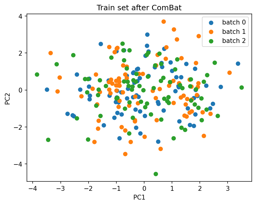
X_train_combat = combat.transform(X_train)
plot_pca(
    X_train_combat.values,
    batch_labels.iloc[X_train_combat.index].values,
    title="Train set after ComBat",
)

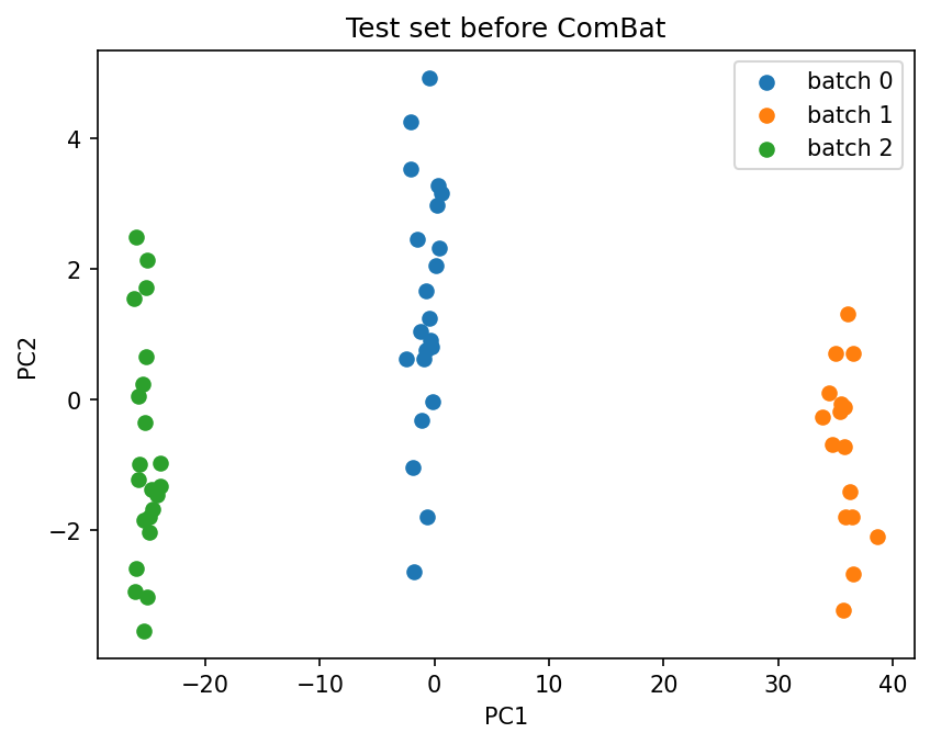
plot_pca(
    X_test.values,
    batch_labels.iloc[X_test.index].values,
    title="Test set before ComBat",
)

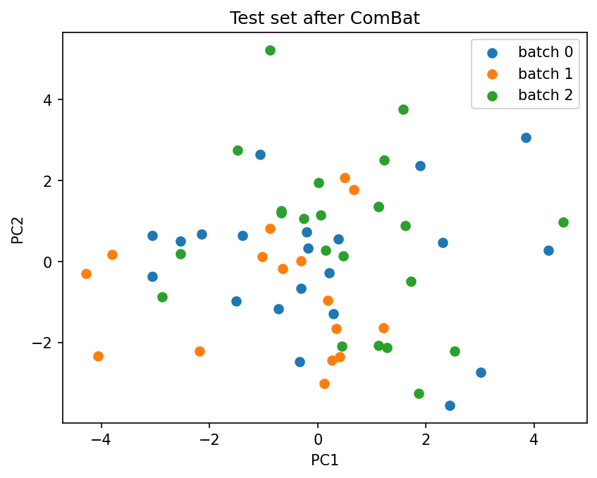
X_test_combat = combat.transform(X_test)
plot_pca(
    X_test_combat.values,
    batch_labels.iloc[X_test_combat.index].values,
    title="Test set after ComBat",
)

Pipeline and cross-validation

pipe = Pipeline(
    [
        ("combat", ComBat(batch=batch_labels, method="johnson")),
        ("scaler", StandardScaler()),
        ("clf", LogisticRegression()),
    ]
)

scores = cross_val_score(pipe, X, y, cv=5)
print(f"Cross-validated accuracy: {scores.mean():.3f} +/- {scores.std():.3f}")

Cross-validated accuracy: 0.903 +/- 0.055

GridSearchCV

pipe_grid = Pipeline(
    [
        ("combat", ComBat(batch=batch_labels, method="fortin", continuous_covariates=age)),
        ("scaler", StandardScaler()),
        ("clf", SVC()),
    ]
)

param_grid = {
    "combat__method": ["johnson", "fortin"],
    "combat__parametric": [True, False],
    "clf__C": [0.1, 1.0, 10.0],
    "clf__kernel": ["linear", "rbf"],
}

grid = GridSearchCV(pipe_grid, param_grid, cv=3, scoring="accuracy", n_jobs=-1)
grid.fit(X, y)

print(f"Best parameters: {grid.best_params_}")
print(f"Best CV accuracy: {grid.best_score_:.3f}")

Best parameters: {'clf__C': 0.1, 'clf__kernel': 'linear', 'combat__method': 'johnson', 'combat__parametric': True}
Best CV accuracy: 0.713

Visualization

combat = ComBat(batch=batch_labels, method="johnson")
combat.fit(X);

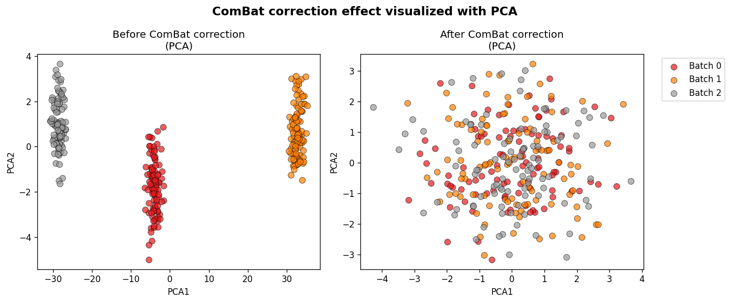
PCA visualization

fig_pca = plot_transformation(combat, X)

UMAP visualization (3D interactive)

plot_transformation(
    combat, X, reduction_method="umap", n_components=3, plot_type="interactive", n_neighbors=30
)

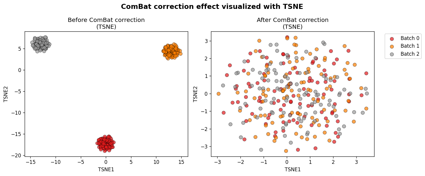
t-SNE visualization (with embeddings)

fig_tsne, embeddings = plot_transformation(
    combat, X, reduction_method="tsne", return_embeddings=True, perplexity=50
)

for k, emb in embeddings.items():
    print(f"{k}: {emb.shape}")

original: (300, 2)
transformed: (300, 2)

Batch Effect Metrics

Quantitatively assess batch correction quality with the compute_batch_metrics() function.

The metrics include:

• Batch effect quantification: Silhouette, Davies-Bouldin, kBET, LISI, variance ratio

• Structure preservation: k-NN preservation, distance correlation

• Alignment metrics: Centroid distance, Levene statistic

By default, metrics are computed in the original feature space. For high-dimensional data, use the pca_components parameter for dimensionality reduction.

combat_metrics = ComBat(batch=batch_labels, method="johnson")
X_corrected = combat_metrics.fit_transform(X)

metrics = compute_batch_metrics(combat_metrics, X)
print(f"Available categories: {list(metrics.keys())}")

Available categories: ['batch_effect', 'preservation', 'alignment']

print("=== Batch Effect Metrics ===")
for name, vals in metrics["batch_effect"].items():
    if name == "lisi":
        print(
            f"{name}: {vals['before']:.3f} -> {vals['after']:.3f} (max: {vals['max_value']})"
        )
    else:
        print(f"{name}: {vals['before']:.3f} -> {vals['after']:.3f}")

=== Batch Effect Metrics ===
silhouette: 0.663 -> -0.006
davies_bouldin: 0.504 -> 82.457
kbet: 0.000 -> 0.987
lisi: 1.000 -> 2.714 (max: 3)
variance_ratio: 1898.114 -> 0.037

print("=== Structure Preservation ===")
print(f"k-NN preservation: {metrics['preservation']['knn']}")
print(f"Distance correlation: {metrics['preservation']['distance_correlation']:.3f}")

print("\n=== Alignment Metrics ===")
for name, vals in metrics["alignment"].items():
    print(f"{name}: {vals['before']:.3f} -> {vals['after']:.3f}")

=== Structure Preservation ===
k-NN preservation: {5: 0.2886666666666666, 10: 0.2876666666666667, 50: 0.3099333333333333}
Distance correlation: 0.122

=== Alignment Metrics ===
centroid_distance: 41.001 -> 0.191
levene_statistic: 0.942 -> 0.183

Using the nn_algorithm parameter

For large datasets, you can choose a specific nearest neighbor algorithm:

metrics_bt = compute_batch_metrics(
    combat_metrics, X, k_neighbors=[5, 10], nn_algorithm="ball_tree"
)
print(f"kBET (ball_tree): {metrics_bt['batch_effect']['kbet']['after']:.3f}")

kBET (ball_tree): 0.987

Metrics on test data

combat = ComBat(batch=batch_labels, method="johnson")
combat.fit(X_train)

test_metrics = compute_batch_metrics(
    combat, X_test, batch=batch_labels.iloc[X_test.index], k_neighbors=[5, 10, 25]
)

print("=== Test Set Metrics ===")
print(
    f"Silhouette: {test_metrics['batch_effect']['silhouette']['before']:.3f} -> {test_metrics['batch_effect']['silhouette']['after']:.3f}"
)
print(
    f"kBET: {test_metrics['batch_effect']['kbet']['before']:.3f} -> {test_metrics['batch_effect']['kbet']['after']:.3f}"
)
print(
    f"Distance correlation: {test_metrics['preservation']['distance_correlation']:.3f}"
)

=== Test Set Metrics ===
Silhouette: 0.656 -> -0.011
kBET: 0.000 -> 0.950
Distance correlation: 0.073

Feature Importance Analysis

Identify which features are most affected by batch effects using the feature_batch_diagnostics() function.

The DataFrame contains three columns:

• location: RMS of batch-specific mean shifts (gamma)

• scale: RMS of log variance changes (log delta)

• combined: Euclidean norm sqrt(location^2 + scale^2)

combat = ComBat(batch=batch_labels, method="johnson")
combat.fit(X)

importance = feature_batch_diagnostics(combat)
print("Top 10 features by batch effect magnitude:")
print(importance.head(10))

Top 10 features by batch effect magnitude:
         location     scale  combined
gene_14  6.775770  0.134143  6.777098
gene_1   6.583819  0.125146  6.585008
gene_10  6.560264  0.190313  6.563024
gene_5   6.535340  0.027457  6.535398
gene_11  6.477399  0.009992  6.477407
gene_8   6.435997  0.023945  6.436042
gene_7   6.376010  0.017880  6.376035
gene_13  6.363834  0.155440  6.365732
gene_3   6.279840  0.051925  6.280055
gene_15  6.238579  0.077490  6.239060

importance_dist = feature_batch_diagnostics(combat, mode="distribution")
print("Top 10 features (relative contribution):")
print(importance_dist.head(10))
print(
    f"\nTop 10 features explain {importance_dist.head(10)['combined'].sum() * 100:.1f}% of total batch effect"
)

Top 10 features (relative contribution):
         location     scale  combined
gene_14  0.051579  0.044349  0.051472
gene_1   0.050117  0.041375  0.050013
gene_10  0.049938  0.062920  0.049846
gene_5   0.049748  0.009078  0.049636
gene_11  0.049307  0.003303  0.049195
gene_8   0.048992  0.007917  0.048881
gene_7   0.048536  0.005911  0.048426
gene_13  0.048443  0.051390  0.048347
gene_3   0.047804  0.017167  0.047697
gene_15  0.047489  0.025619  0.047385

Top 10 features explain 49.1% of total batch effect

Visualizing feature importance

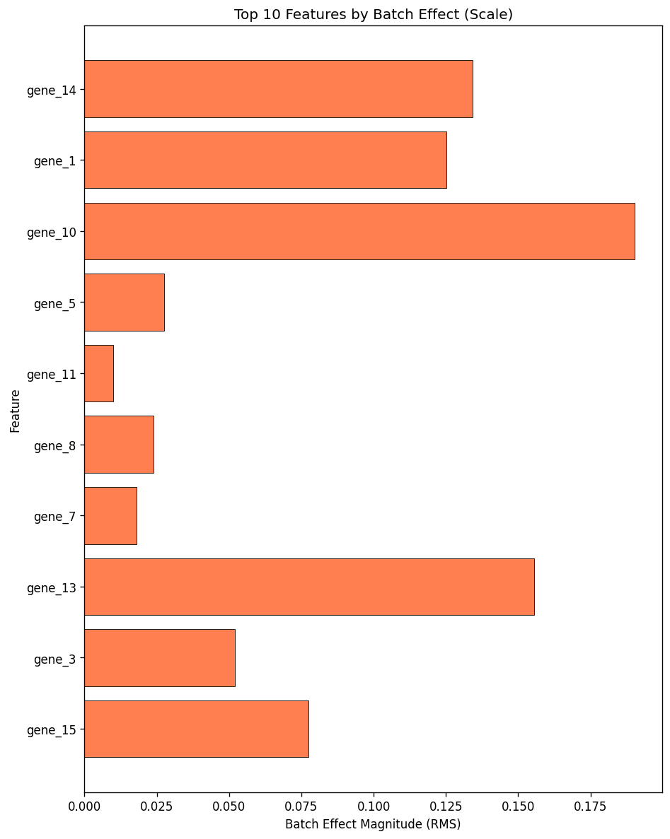
fig = plot_feature_diagnostics(combat, top_n=10, kind="combined", mode="magnitude")

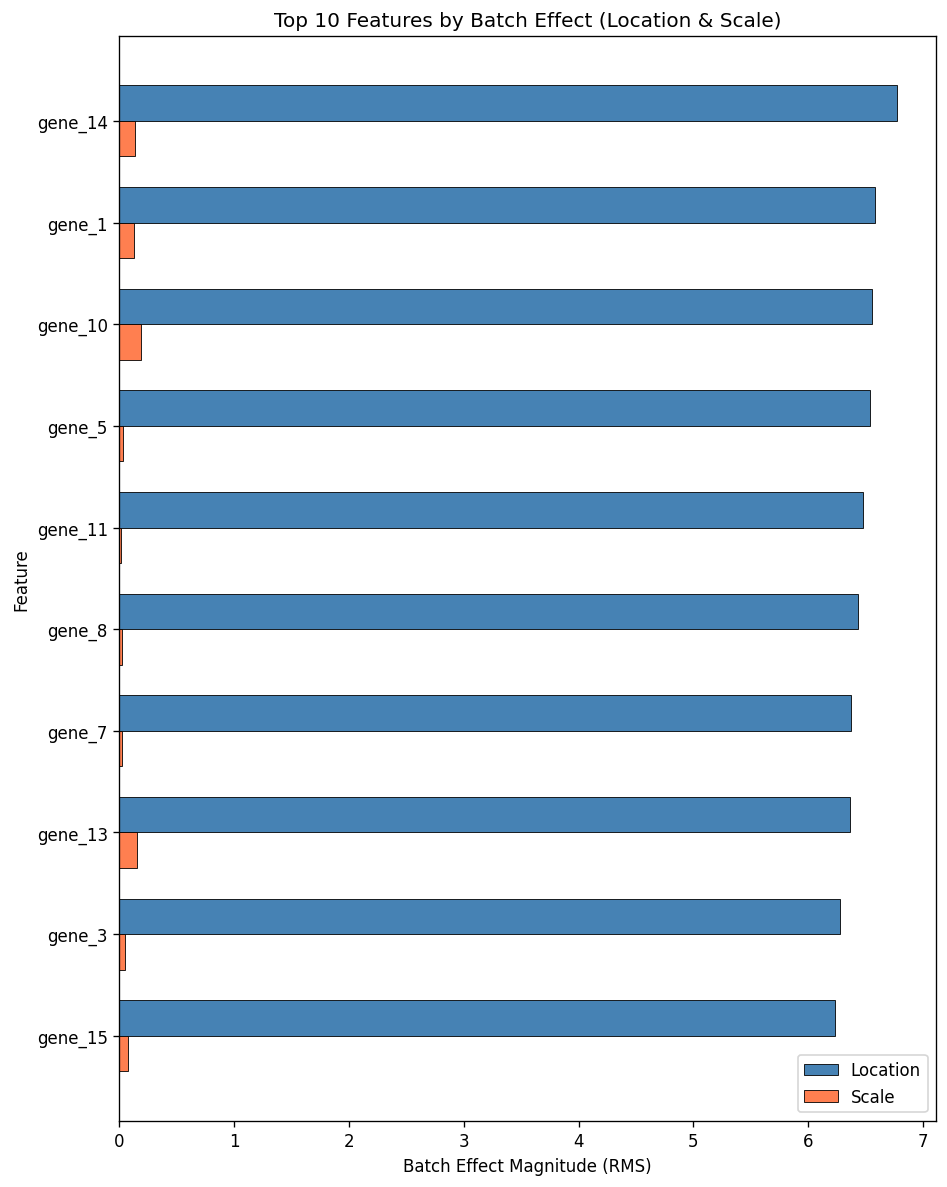
For kind="combined", the layout="diverging" option draws location and scale as back-to-back bars, each with its own x-axis and grid, while keeping the absolute magnitudes. This is clearer than the shared-axis grouped plot above when one component dominates the other: here the scale RMS is far smaller than the location RMS, so the scale bars are nearly invisible in the grouped plot but readable once they have their own axis.

fig = plot_feature_diagnostics(combat, top_n=10, kind="combined", mode="magnitude", layout="diverging")

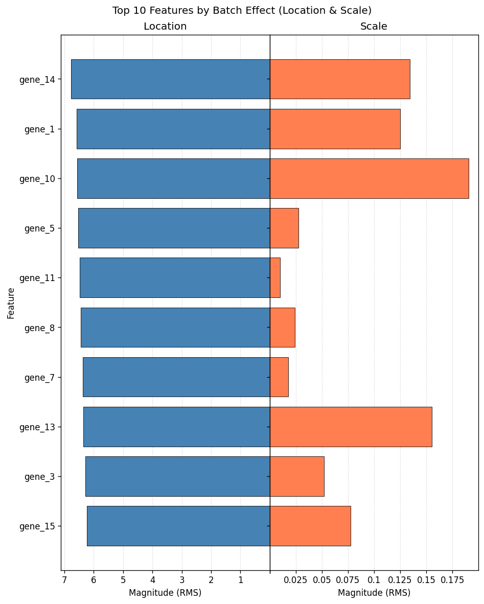
fig = plot_feature_diagnostics(combat, top_n=10, kind="combined", mode="distribution")

Top 10 features explain 49.1% of total batch effect

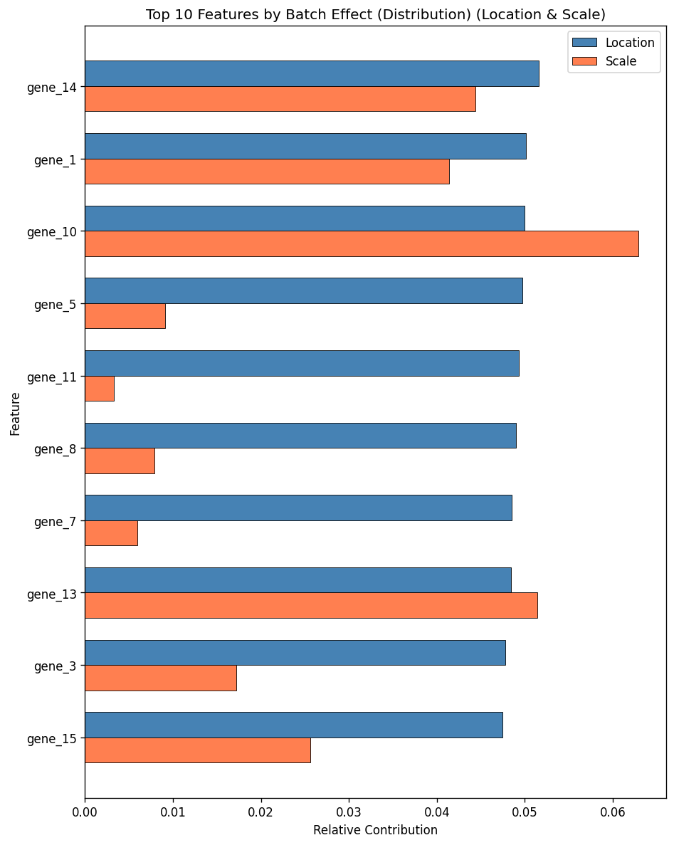
fig = plot_feature_diagnostics(combat, top_n=10, kind="location")

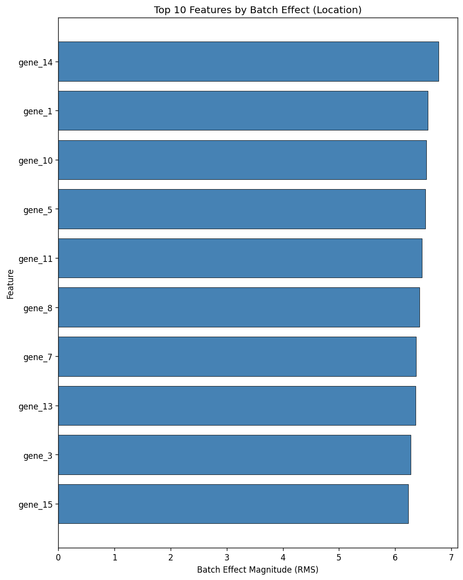
fig = plot_feature_diagnostics(combat, top_n=10, kind="scale")

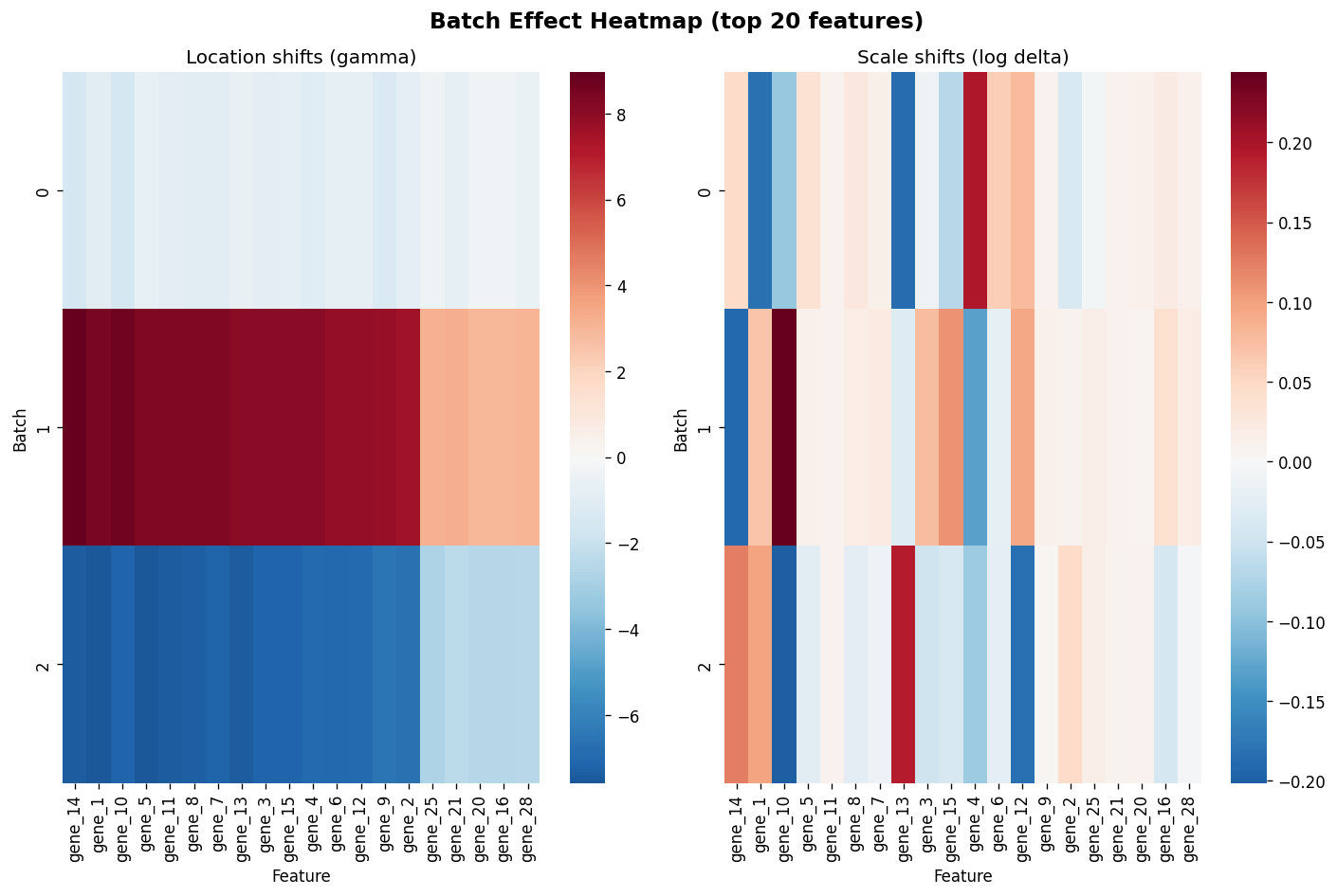
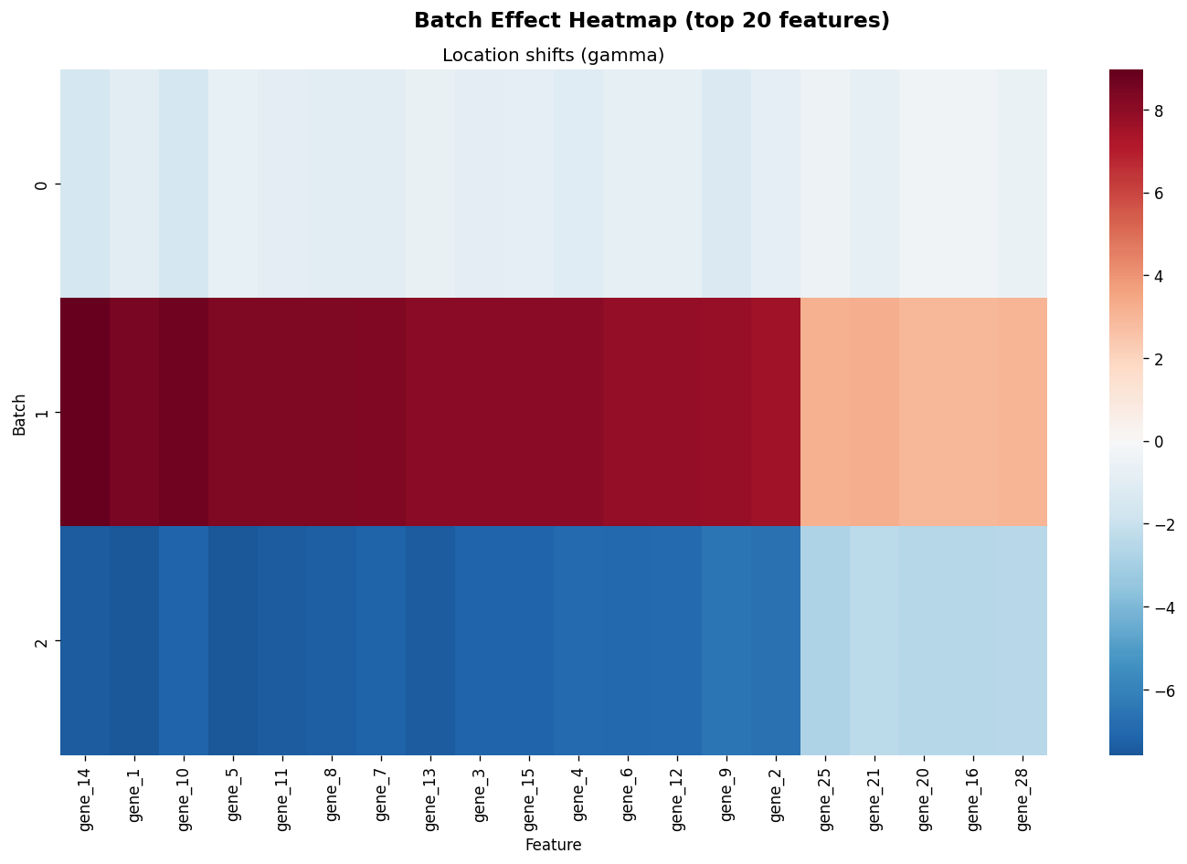
Batch Effect Heatmap

The plot_batch_effect_heatmap() function shows the estimated batch-specific location shifts (gamma) and log-scale shifts (log delta) for the top features.

fig = plot_batch_effect_heatmap(combat, top_n=20)

combat_mo = ComBat(batch=batch_labels, method="johnson", mean_only=True)
combat_mo.fit(X)

fig = plot_batch_effect_heatmap(combat_mo, top_n=20)

Model Summary

The summary() function provides a human-readable diagnostic report after fitting.

combat = ComBat(batch=batch_labels, method="fortin", discrete_covariates=sex, continuous_covariates=age)
combat.fit(X)

print(summary(combat))

ComBat Summary
========================================
Method:          fortin
Parametric:      True
Mean only:       False
Reference batch: None
Number of batches: 3
Samples per batch:
  0: 100
  1: 100
  2: 100
Number of features: 50

Top 5 features by batch effect (combined):
  gene_14: 6.8059
  gene_10: 6.6371
  gene_1: 6.5902
  gene_5: 6.5382
  gene_11: 6.4846

Diagnostics
========================================
Metric                            Value
------                            -----
Batch var. explained (before)     92.7%
Design matrix condition number    279.4
EB convergence (parametric):
  0                               converged (2 iter)
  1                               converged (2 iter)
  2                               converged (2 iter)

sklearn set_output API

ComBat supports the get_feature_names_out() method, enabling the sklearn set_output API for automatic pandas output in pipelines.

combat = ComBat(batch=batch_labels, method="johnson")
combat.fit(X)

print("Feature names out:", combat.get_feature_names_out()[:5], "...")

Feature names out: ['gene_1' 'gene_2' 'gene_3' 'gene_4' 'gene_5'] ...

pipe = Pipeline(
    [
        ("combat", ComBat(batch=batch_labels, method="johnson")),
        ("scaler", StandardScaler()),
    ]
)
pipe.set_output(transform="pandas")

result = pipe.fit_transform(X)
print(type(result))
print(result.columns[:5].tolist(), "...")
result.head()

<class 'pandas.core.frame.DataFrame'>
['gene_1', 'gene_2', 'gene_3', 'gene_4', 'gene_5'] ...

	gene_1	gene_2	gene_3	gene_4	gene_5	gene_6	gene_7	gene_8	gene_9	gene_10	...	gene_41	gene_42	gene_43	gene_44	gene_45	gene_46	gene_47	gene_48	gene_49	gene_50
0	0.420532	-1.126626	0.728137	0.875776	-2.064081	-1.192271	0.132254	-0.422611	0.037988	-0.813113	...	0.737502	0.417632	-0.523629	0.436567	0.097437	0.336822	0.766864	0.275114	0.673753	0.061233
1	0.402138	0.580830	-1.557645	-0.292021	-0.534927	-0.573265	-0.284690	1.462481	-0.805589	1.303593	...	0.663535	-0.181029	-0.284341	0.124122	-1.799768	-1.310010	-1.345514	-0.916274	0.395693	-0.878495
2	-0.384767	1.263231	-0.417769	0.687621	-1.013344	-0.168769	-0.982951	-0.446332	0.889592	-1.829180	...	0.425134	-1.012396	-1.972466	0.472182	-0.880209	-0.290004	-0.661387	-0.080481	1.059324	0.147638
3	-0.125885	-1.122202	-1.782875	-0.446434	-0.104694	1.672817	0.134772	0.929378	-0.441408	-1.198840	...	1.668792	-0.256635	-0.244714	1.668080	-1.189505	-0.763915	0.547261	-0.328172	-0.007638	-0.161876
4	0.459279	1.373828	0.044904	0.600908	-2.166465	-0.022516	-0.872460	-1.362013	-0.817831	-0.210033	...	-0.801440	-0.177089	-1.602666	-1.265722	2.213954	-1.152138	-1.128017	1.849510	2.891302	-1.135469

5 rows × 50 columns